2) Using multiple cores via the parallel package
Parallel Package
This package provides the mechanisms to support "core-grained" parallelism. Large portions of code can run concurrently with the objective to reduce the total time for the computation. Many of the package routines are directed at running the same function many times in parallel. These functions do not share data and do not communicate with each other. The functions can take varying amounts fo time to execute, but for best performance should be run in similar time frames.
The computational module used by the Parallel package is:
- Initialise "worker" processes
- Divide users task into a number of sub-tasks
- Allocate the task to workers
- Wait for tasks to complete
- If task still waiting to be processed goto 3
- Close down worker processes
Additional documentation for the parallel package
doParallel package and "foreach"
Parallel Package Functions
library(parallel)
makeCluster(<size of pool>)
stopCluster(cl)
The foreach function allows general iteration over elements in a collection without the use of an explicit loop counter. Using foreach without side effects also facilitates executing the loop in parallel.
w <- foreach(i=1:3) %dopar% sqrt(i)
x <- foreach(a=1:3, b=rep(10, 3)) %do% (a + b)
y <- foreach(seq(from=0.5, to=1, by=0.05), .combine='c') %dopar% exp(i)
z <- foreach(seq(from=0.5, to=1, by=0.05), .combine='cbind') %dopar% rnorm(6)

> w
[[1]]
[1] 1
[[2]]
[1] 1.414214
[[3]]
[1] 1.732051
> x
[[1]]
[1] 11
[[2]]
[1] 12
[[3]]
[1] 13
> y
 [1] 54.59815 54.59815 54.59815 54.59815 54.59815 54.59815 54.59815 54.59815 54.59815 54.59815 54.59815
> z
       result.1  result.2   result.3   result.4   result.5    result.6   result.7   result.8    result.9
[1,]  0.8993342 1.1204134 -0.2309854 -0.5671736 -0.3717168  0.48318550  1.0714748  2.7472543 -0.27836383
[2,] -5.0370385 0.9198819  2.1315785  0.3508126  1.0994210  0.84825381  1.4797737  0.4806012 -1.12378917
[3,]  2.5562184 0.1189899 -0.8148065 -0.3892018 -0.7672944 -0.57028899 -1.2352417  0.2983788  0.05779129
[4,] -0.6017708 0.1937990  1.4447131 -0.5821553 -1.9262707  1.08985089  0.1355017 -1.6901487 -0.84403261
[5,] -0.1641378 1.2524972 -1.2568069  0.9968563 -1.0173397 -0.01730798 -0.7163426 -0.5800342 -1.90478362
[6,] -1.2754269 0.1144449 -2.7935687 -1.0767441  0.2387643 -0.62121996  0.8327163 -1.5710432 -2.39983048
      result.10  result.11
[1,] -0.7757645 -1.3728983
[2,] -0.4399470 -0.8827042
[3,] -0.3680583 -0.9994829
[4,]  0.7126810 -1.0699761
[5,]  0.6203577  0.2573745
[6,] -0.1223131 -1.3356456
Additional documentation for doParallel package and iterators package.
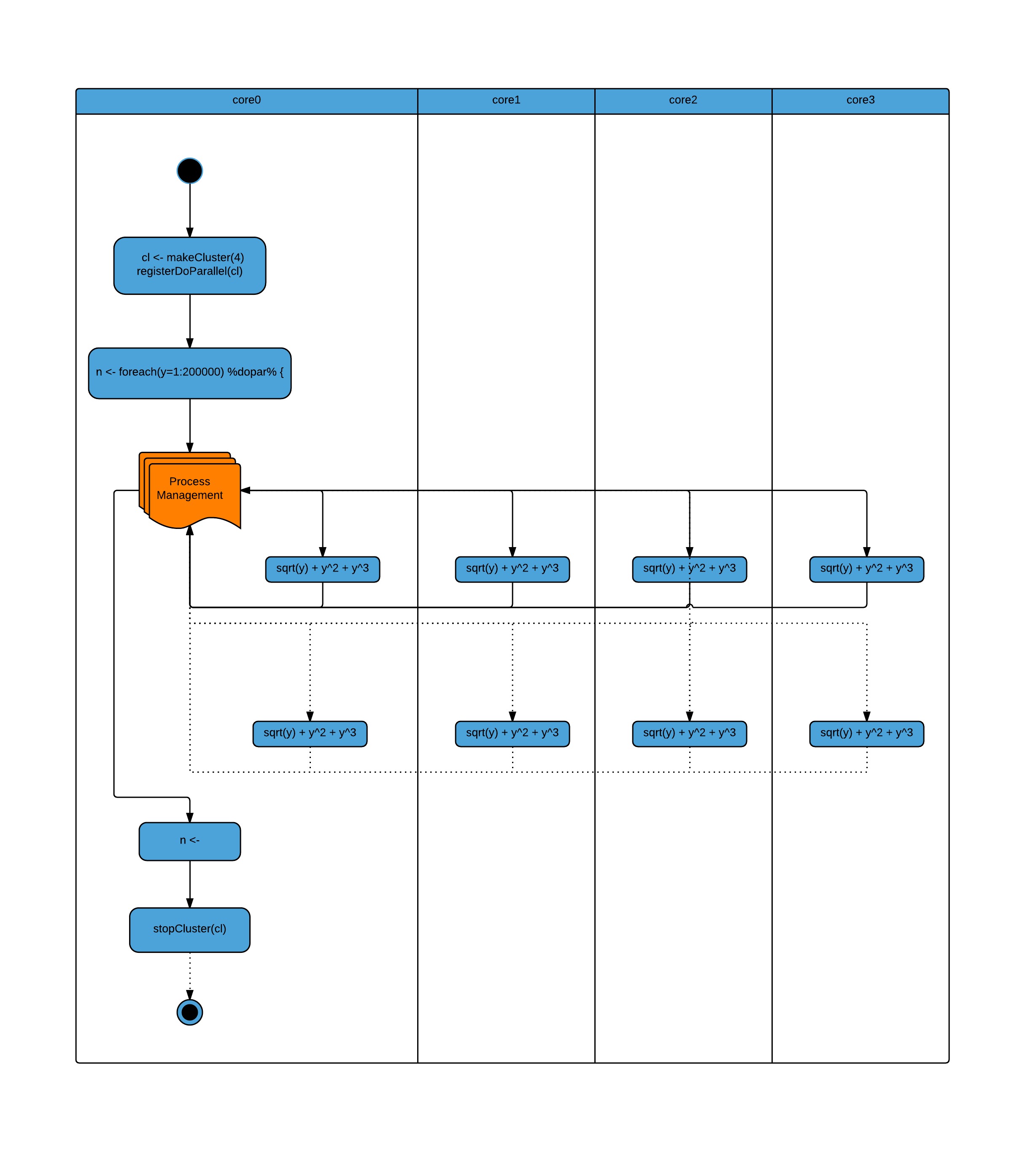
library(doParallel)

# simple example
foreach.example <- function(procs) {

  cl <- makeCluster(procs)
  registerDoParallel(cl)

  #start time
  strt<-Sys.time()

  n <- foreach(y=1:200000) %dopar% {

    sqrt(y) + y^2 + y^3

  }

  # time taken
  print(Sys.time()-strt)

  stopCluster(cl)

}
> foreach.example(1)
Time difference of 2.060153 mins
> foreach.example(2)
Time difference of 1.479866 mins
> foreach.example(4)
Time difference of 1.831992 mins
Running the function over two cores has improved the performance, but on four cores it's slowed down. This is because the function is not doing very much work and the overhead of managing the worker processes is greater than the work being done.
Here is a more substantial example:
foreach.heavy.example <- function(procs) {

  cl <- makeCluster(procs)
  registerDoParallel(cl)

  #start time
  strt<-Sys.time()

  n <- foreach(y=1:20) %dopar% {

    a <- rnorm(500000)
    summary(a)
    min(a); max(a)
    range(a)
    mean(a); median(a)
    sd(a); mad(a)
    IQR(a)
    quantile(a)
    quantile(a, c(1, 3)/4)

  }

  # time taken
  print(Sys.time()-strt)

  stopCluster(cl)

}
> compare <- microbenchmark(foreach.heavy.bm(1), foreach.heavy.bm(2), foreach.heavy.bm(3), foreach.heavy.bm(4), times = 20)
> autoplot(compare)
> foreach.heavy.example(1)
Time difference of 5.73893 secs
> foreach.heavy.example(2)
Time difference of 3.093377 secs
> foreach.heavy.example(3)
Time difference of 2.345401 secs
> foreach.heavy.example(4)
Time difference of 1.868922 secs
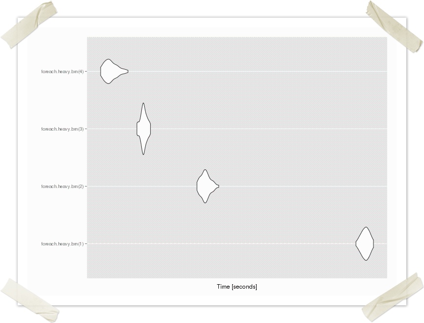
The graph shows the time for execution of 50 trials for 1 - 4 processes (cores).
Beware Hyper-threading
To quote Wikipedia:
Hyper-threading
Hyper-Threading Technology is a form of simultaneous multithreading technology introduced by Intel. Architecturally, a processor with Hyper-Threading Technology consists of two logical processors per core, each of which has its own processor architectural state. Each logical processor can be individually halted, interrupted or directed to execute a specified thread, independently from the other logical processor sharing the same physical core.[4]
Unlike a traditional dual-core processor configuration that uses two separate physical processors, the logical processors in a Hyper-Threaded core share the execution resources. These resources include the execution engine, the caches, the system-bus interface and the firmware. These shared resources allow the two logical processors to work with each other more efficiently, and lets one borrow resources from the other when one is stalled. A processor stalls when it is waiting for data it has sent for so it can finish processing the present thread. The degree of benefit seen when using a hyper-threaded or multi core processor depends on the needs of the software, and how well it and the operating system are written to manage the processor efficiently.[4]
Hyper-threading works by duplicating certain sections of the processor—those that store the architectural state—but not duplicating the main execution resources. This allows a hyper-threading processor to appear as the usual "physical" processor and an extra "logical" processor to the host operating system (HTT-unaware operating systems see two "physical" processors), allowing the operating system to schedule two threads or processes simultaneously and appropriately. When execution resources would not be used by the current task in a processor without hyper-threading, and especially when the processor is stalled, a hyper-threading equipped processor can use those execution resources to execute another scheduled task. (The processor may stall due to a cache miss, branch misprediction, or data dependency.)
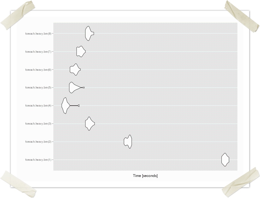
The graph below show the effects of hyper-threading on an "8 core" laptop. Only 4 cores are of use. Switch it off and use only the real cores.
Parallel "apply" functions
Parallel Package Functions
parLapply(cl = NULL, X, fun, ...)
parSapply(cl = NULL, X, FUN, ..., simplify = TRUE, USE.NAMES = TRUE)
parApply(cl = NULL, X, MARGIN, FUN, ...)
parRapply(cl = NULL, x, FUN, ...)
parCapply(cl = NULL, x, FUN, ...)
| Description | base function | Parallel Package |
|---|---|---|
Apply Functions Over Array Margins returns a vector, array, or list | apply | parApply |
Apply a Function over a List or Vector returns a list | lapply | parLapply |
Apply a Function over a List or Vector returns a vector, matrix or array | sapply | parSapply |
Apply a Function over a row or column of a matrix | parRapply parCapply |
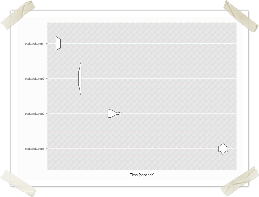
parLapply example
library(parallel)

apply.function <- function(data) {

  summary(data)
  min(data); max(data)
  range(data)
  mean(data); median(data)
  sd(data); mad(data)
  IQR(data)
  quantile(data)
  quantile(data, c(1, 3)/4)

}

apply.example <- function(procs) {

  cl <- makeCluster(procs)
  registerDoParallel(cl)

  data.list <- replicate(10, rnorm(5000000), simplify=FALSE)

  #start time
  strt<-Sys.time()

  parLapply(cl, data.list, apply.function)

  # time taken
  print(Sys.time()-strt)

  stopCluster(cl)

}
> apply.example(1)
Time difference of 21.74148 secs
> apply.example(2)
Time difference of 11.06617 secs
> apply.example(3)
Time difference of 9.244002 secs
> apply.example(4)
Time difference of 7.421883 secs
>